Program Language - R ( 제조업 프로세스에서 활용 )

Data manipulation
Plot
Statistics

t.test

t.test

ANOVA

MANOVA

ANCOVA

RM-ANOVA

Reliability

PCA

Correlation

Linear Regression

Discriminant Analysis

Clustering Analysis

Machine Learning

프로세스별 활용

R 은 통계분석을 위한 아주 유용한 Open source 프로그램이다. 배우기도 용이하고 무엇보다 Open source 프로그램 이기에 비용 부담도 없다는 것이다. 제조기업 현장에서 통계분석이 필요한 여러가지 상황에서 사용할 수 있는 방법을 제시하고자 한다.

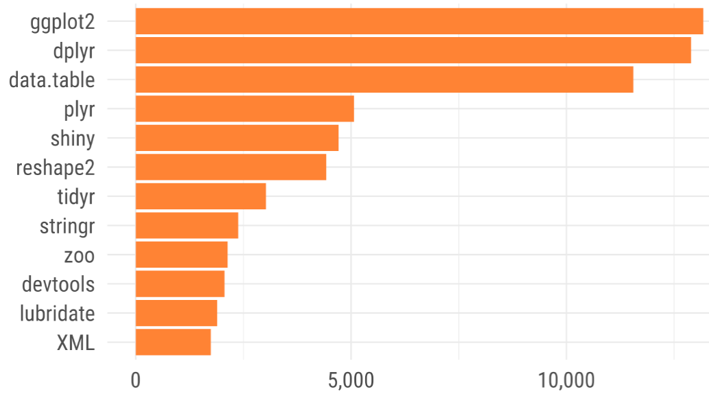
image source : https://statkclee.github.io/data-science/data-science-library.html

Data manipulation

R 설치 : https://www.r-project.org/

개발도구 : RStudio : https://www.rstudio.com/

개발도구 : atom : https://atom.io/

Data type : vector, data.frame, matrix, list

비교와 블리언

논리 연산 / 변수 /주석 처리

제어 & Function

data.frame / matrix

read.table(), cbind, rbind

do.call(rbind, mylist)

merge , append(list_x, list(x=10, y=20))

Plot : Bart, Histogram, Scree Chart

t 검정, 분산분석, 요인분석

일, 독립표본 : t.test( dataset , mu=170)

대응 표본 : t.test (d, paired = T, var.equal=T)

등분산 검정 : var.test( v1, v2 )

분산분석 : aov( score ~ gender + class + gender : class)

PCA : 다중공선성 Check - cor(), data 편향시 log(),

prcomp(d, center=T, scale. = T )

결과 해석

회귀분석 : lm( label ~ PC1 + PC2, data = )

예측 및 성능 확인

신뢰도 분석 : library(ltm, psy) / alpha(Q)

독립성 분석 : data.frame(class * score),

chisq.test (dt)

동질성 분석 : chisq.test (dt)

적합도 분석 : chisq.test (obs, p=prob)

편상관 분석

plot(pressure ~ temperature, data = pressure)

분류분석 (회귀, 판별, 군집)

회귀분석 : lm()

Logistics : aod : wald.test

glm(~ , family="binomial")

판별분석 : lda( y ~ . , ... )

prior ; 사전확률 /predict(~ , )

집단평균의 동질성 검정,

Wilks’ lamda, 정준판별함수,

고유값, 정준판별함수 계수,

분류함수계수

clustering : hclust(dist(iris[, 3:4]))

plot(clu) / cutree(clu, 3)

table(clu_cut, iris$Species)/

kmeans : library(caret) / train, test datase split

kmeans(training_data[,-5], centers = 3, iter.max = 10000)

table(training$Species, training$cluster)

non-parametric : wilcox.test(A, B, paired = FALSE, alternative = "two.sided", mu = 0.0, exact = TRUE, correct = TRUE, conf.int = TRUE, conf.level = 0.95)

mann whitney / PLOT

Data type

code 참조 : github

Data type : vector, data frame, matrix(array), factor, list

자료형 확인 및 정의 : as.character(x), as.complex(x) , as.numeric(x) or as.double(x), as.integer(x), as.logical(x)

vector : 백터는 동질적dls 같은 자료형으로 같은 모드를 가지고 있어야 한다. 하나의 값으로 구성된 백터가 스칼라이고 여러개 있으면 벡터

data frame : 데이터를 열을 기준으로 정리한 것으로 표 형태의 데이터를 표현하기 위함이다. x <- 1:10 # mean(x) # sd(x) # var(x)

행은 모두 같은 길이이며, 열은 하나의 엘리먼트를 나타낸다. 행렬과 다른점은 각각의 행들이 서로다른 데이터 타입들을 가질 수 있다는 것이다. 즉, 각각의 열들은 같은 타입으로 이뤄지지만, 모든 열이 모두 같을 필요는 없다. data.matrix() : 행렬을 data frame으로 변경 할 수 있다.

데이터 프레임 합치기는 cbind # 두개의 데이터를 열로 쌓고, rbind # 두개의 데이터를 행으로 쌓는다.

matrix(array) : vector 에 차원을 정해준 것이 바로 Matrix이다. 백터의 dim 속성이 처음엔 NULL 이지만 이것을 주게 되면 matrix가 된다.

dim(2,3) # 2 by 3 행렬 / Array (배열) 3차원 matrix 부터는 배열이라는 이름을 쓴다.

Factor(요인) : 요인들은 간단하고 효율적인 형태로 데이터 프레임에 저장되어 특별한 속성이 있다. R은 백터에 있는 고유한 값(unique value)의 정보를 얻어 내는데, 이 고유 값들을 요인의 '수준(level)'이라고 일컫는다. 요인의 범주형 변수 기능으로, 분할표, 선형 회귀, 변량 분석, 로지스틱 회귀 분석에 사용 된다. 집단 분류 기능은 데이터 항목에 라벨을 붙이거나 태깅을 할 때 쓰는 방법이다.factor( x, levels, ordered #TRUE=순서형, FALSE=명목형 데이터) / nlevels(x) / 중간에 값 넣기 ; factor(append(as.character(gender),"TRUE"))

list : 이질적인 다양한 자료형을 포함 할수 있다. 연속적인 리스트라면, do.call(rbind,mylist) 이용 모두 행열이 같은 크기일때만 가능하다. 서로다른 데이터 프레임 합치기는 merge 일치하는 부분만 합치고 싶으면, merge(A,B, by="열 이름") 으로 설정한다.

Data manipulation

( source code 참조 ) 수와 계산 : / 변수 : / 제어 : / 비교와 블리언 : / 조건문 : / 입력과 출력 : / 논리 연산 : / Plot/ Bart chart /. Histogram / Scree Chart / 자료형 확인 및 정의 : as.character(x), as.complex(x) , as.numeric(x) or as.double(x)

data handling : rm(list = ls()) / # vector x1 <- c(1,2,3) x <- 1:9 x x1 <- c(1: 9) n1 <- rep(10,3) n1 <- rep(1:3, 3) n1 x1.n1 <- data.frame(x1, n1) x1.n1

data.frame, matrix : row.names(df2) , data.matrix()
# read.table(), read.csv() / # list -> data.frame / data.frame(list_x) : a <- data.frame(1:3, 11:13) / a$X1.3 / grep(2,a[,2]) / grep("X1.3",colnames(a)) / names(a) / names(a) <- c("hd1", "hd2") / names(a)[names(a)=="hd1"] <- c("newhd")

a$newcol <- NA / a$badcol <- NULL / subset(a, select = -newcol) / cbind, rbind/ do.call(rbind, mylist) / merge (df1, df2, by = intersect(names(df1),names(df2)))

list : no <- c(1:3) / name <- c("a", "b", "c") / weight <- c(50, 60, 70) / df1 <- data.frame(no, name, weight)

list_x <- list(x, df1) / list_y <- list(me=c(1:3), sd =0.5, center=0) / list_y$me[2] / list_y$me[-c(2,3)] / list_y <- list(list_y, list_x)

emty_list <- list.files("./var1/") / filenames <- sapply(emty_list,list)
# Foreach , # .final/ # compare data.frame /tem <- 1:3/ names(tem) <- c("hd1", "hd2", "hd3") / mode(tem) / df2 <- data.frame(x=1:3, y=c("aa","bb","cc")) / mode(df2) / append(list_x, list(x=10, y=20)) / append(list_x, list(f=1:5), after=0)

Function : rnorm_fixed = function(n, mu=0, sigma=1) { x = rnorm(n) # from standard normal distribution x = sigma * x / sd(x) # scale to desired SD x = x - mean(x) + mu # center around desired mean return(x) }

t.test

a = c(175, 168, 168, 190, 156, 181, 182, 175, 174, 179) / b = c(185, 169, 173, 173, 188, 186, 175, 174, 179, 180) / var.test(a,b) / t.test(a, mu=170)

요인 분석

주성분 분석과 공통요인 분석으로 구분된다.

#1. multicollinearity check : cor(iris[1:4]) ; # some of them are big as 0.87

# 2. biased data -> transform log / log_ir <- log(iris[, 1:4]) 데이터가 편향된 경우 사용 (skip도 가능) / ir_species <- iris[,5]

# 3. pca analysis : # Unlike princomp, prcomp : variances are computed with the usual divisor N - 1. ir_pca <- prcomp(log_ir, center = T, scale. = T) train, test dataset 으로 구분하여 성능 확인도 가능

# 4. plot scree graph : plot(ir_pca,type="lines")

# 5. summary : check that how much it has a power of explanation Cumulative Proportion summary(ir_pca)/ # Cumulative Proportion 0.7331 of PC1, 0.9599 with PC2

# 6. linear regression : prc <- as.matrix(log_ir) %*% ir_pca$rotation # skip 가능

# 7. train <- cbind(ir_species,as.data.frame(prc)) train[,1] <- as.factor(train[,1]) / colnames(train)[1] <- "label"

# 8. linear regression with PC1, PC2 / fit <- lm(label~PC1+PC2, data=train)

# 9. performance check / fit_pred <- predict(fit, newdata = train)

# 10. comparision the both prediction, actual / b <- round(fit_pred) / b[b==1] <- "setosa" / b[b==2] <- "Versicolor" / b[b==3] <- "Virginica" / a <- ir_species / table(b,a)

신뢰도 분석

# 1. data : Q <- data.frame( Q1=c(1,4,2,3,4,2,3,4,3,2), Q2=c(2,4,1,2,4,1,2,5,2,1), Q3=c(2,5,1,3,3,2,3,4,2,2)) / pairs(Q, panel=panel.smooth)

# 2. cronbach : alpha () : library(psy) / cronbach(Q) : library(psych) / a <- alpha(Q) / a$total / View(a$scores)

Correlation

Spearman's correlation : / 독립성 분석 : / 동질성 분석 : / 적합도 분석

# 1. aq <- airquality[,c(1:4)] / cor(aq) / aq2 <- na.omit(aq) / cor(aq2) / plot(aq2) / pairs(aq2, panel=panel.smooth

# 2. library(PerformanceAnalytics) / chart.Correlation(aq2, histogram=TRUE, pch=19)

# 3. library(corrplot) / aq.cor <- cor(aq2) / corrplot(aq.cor, method="number")

## 1. goodness of fit test : chisq.test() / obs <- c(19, 40, 35) / prob <- c(2/10, 3/10, 5/10) / chisq.test(obs, p=prob)

## indexing / chisq.test() of data from data frame / # chisq.test() of data from data frame / data(Cars93, package="MASS") / Car_Type <- table(Cars93$Type)

# Car_Type_Prob <- c(0.2, 0.1, 0.2, 0.2, 0.2, 0.1) / chisq.test(x=Car_Type, p=Car_Type_Prob)

## b. test of independence / # data key-in way 1 : rbind() row_1 <- c(7, 13, 9, 12) / row_2 <- c(13, 21, 10, 19) / row_3 <- c(11, 18, 12, 13) / data_rbind <- rbind(row_1, row_2, row_3)

# data key-in way 2 : matrix() / raw_data <- c(7, 13, 9, 12, 13, 21, 10, 19, 11, 18, 12, 13) / dt <- matrix(raw_data, byrow=TRUE, nrow=3)

# giving names to the rows and columns of the data table : dimnames() / dimnames(dt) <- list("Class" = c("Class_1", "Class_2", "Class_3"), "Score" = c("Score_H", "Score_M", "Score_L", "Fail"))

## exploratory data analysis / # marginal distribution : addmargins() / addmargins(dt) / prop.table(dt)

addmargins(prop.table(dt)) / # bar plot : barplot(t(dt), beside=TRUE, legend=TRUE, ylim=c(0, 30), ylab="Observed frequencies in sample", main="Frequency of math score by class")

# indexing statistics of chisq.test() / fit <- chisq.test(dt) / fit$observed # observed frequency / fit$expected # expected frequeycy /

fit$residuals # residual between observed and expected frequecy / fit$statistic # chi-squared statistics / fit$parameter # degrees of freedomfit / fit$p.value # P-value

## c. test of homogeneity : raw_data <- c(10, 20, 30, 10, 40, 30) / dt <- matrix(raw_data, byrow=TRUE, nrow=2) / # giving names : dimnames(dt) <- list("Gender" = c("f", "m"), "par" = c("aa", "bb", "cc"))

## exploratory data analysis # marginal distribution : addmargins() addmargins(dt) # proportional distribution : prop.table() prop.table(dt) addmargins(prop.table(dt))

# bar plot : barplot(t(dt), beside=TRUE, legend=TRUE, ylim=c(0, 120), ylab="Observed frequencies ", main="Parament preferences by gender")

## chisquared test : chisq.test(dt) # indexing statistics of chisq.test() / fit <- chisq.test(dt) / fit$observed # observed frequency / fit$expected # expected frequeycy

fit$residuals # residual between observed and expected frequecy / fit$statistic # chi-squared statistics / fit$parameter # degrees of freedomfit / fit$p.value

Logistic classification

이분 분류형에 대한 : .....

# logistics regression : dataset ready -> xtabs : d <- data.frame(x=c("1", "2", "2", "1"), y=c("A", "B", "A", "B"), num=c(3, 5, 8, 7))
xtabs(num ~ x + y, data=d)

# 1. library(ggplot2) mydata <- read.csv("https://stats.idre.ucla.edu/stat/data/binary.csv")

sapply(mydata, sd) / # contingency table : xtabs(~ x + y, data) xtabs(~admit+rank, data=mydata)

# factor : mydata$rank <- factor(mydata$rank) mylogit <- glm(admit ~ gre + gpa + rank, data = mydata, family = "binomial") summary(mylogit)

## aod : walt.test / library(aod) wald.test(b = coef(mylogit), Sigma = vcov(mylogit), Terms = 4:6)

# OR 비 : exp(coef(mylogit)) / newdata1 <- with(mydata, data.frame(gre = mean(gre), gpa = mean(gpa), rank = factor(1:4)))

# rank, gpa 고정후 : newdata2 <- with(mydata, data.frame(gre = rep(seq(from = 200, to = 800, length.out = 100), 4), gpa = mean(gpa), rank = factor(rep(1:4, each = 100))))

# rank : newdata3 <- cbind(newdata2, predict(mylogit, newdata = newdata2, type = "link", se = TRUE)) newdata3 <- within(newdata3, { PredictedProb <- plogis(fit) LL <- plogis(fit - (1.96 * se.fit)) UL <- plogis(fit + (1.96 * se.fit)) })

ggplot(newdata3, aes(x = gre, y = PredictedProb), geom_ribbon(aes(ymin = LL, ymax = UL, fill = rank),alpha = 0.2), geom_line(aes(colour = rank))) ggplot(newdata3, aes(x = gre, y = PredictedProb))

reference site

Dummy Linear Regression / Hierarchical analysis / Logistics Regression
Mediation Regressions / Moderator Regressions

Discriminant analysis

판별분석은 집단으로 구분되는 종속변수와 독립변수를 가지고 하는 분석

# 1. dataset : set.seed(123) aa_length <- sample(seq(15,22.5,by=0.5), 50, replace=T) aa_weight <- sample(seq(0.2,0.8,by=0.05), 50, replace=T) bb_length <- sample(seq(46,61,by=0.5), 50, replace=T) bb_weight <- sample(seq(1.36,3.2,by=0.5), 50, replace=T) cc_length <- sample(seq(30,75.5,by=1), 50, replace=T)

cc_weight <- sample(seq(0.2,3.5,by=0.1), 50, replace=T) dd_length <- sample(seq(25,38,by=0.5), 50, replace=T) dd_weight <- sample(seq(0.4,0.54,by=0.01), 50, replace=T) ee_length <- sample(seq(22,55,by=0.5), 50, replace=T) ee_weight <- sample(seq(0.68,1.8,by=0.01), 50, replace=T)

length <- c(aa_length, bb_length, cc_length, dd_length, ee_length) weight <- c(aa_weight, bb_weight, cc_weight, dd_weight, ee_weight) speed <- rnorm(50*5, 7.2, sd=1.8)

fish <- c(rep("aa",50), rep("bb", 50), rep("cc", 50), rep("dd", 50), rep("ee", 50)) fish_data <- data.frame(length, weight, speed, fish)

## 2. lda : library(MASS) / fish_lda <- lda(fish ~., data=fish_data, prior=c(1,1,1,1,1)/5) / fish.lda$counts

set.seed(123) / train100 <- sample(1:nrow(fish_data),100) table(fish_data$fish[train100]) fish100_lda <- lda(fish ~., data=fish_data, prior=c(1,1,1,1,1)/5, subset=train100)

## predict() : predict_fish100 <- predict(fish100_lda) table(fish_data$fish[train100], predict_fish100$class)

# ggplot() : library(ggplot2) p <- ggplot(as.data.frame(predict_fish100$x), aes(x=LD1, y=LD2, col-fish_data$fish[train100])) p <- p + geom_point() + geom_text(aes(label=as.character(predict_fish100$class))) # Adjust legend size

<- p + theme(legend.title=element_blank(), legend.text=element_text(size=20, face="bold")) # Adjust axis labels p <- p + theme(axis.title=element_text(face="bold", size=20), axis.text=element_text(size=18)) # Display plot

## misclassficaiotn rate : predict_new <- predict(fish100_lda, newdata=fish_data[-train100,]) table(fish_data$fish[-train100], predict_new$class) / tab <- table(fish_data$fish[-train100], predict_new$class)

## error rate / tab_sum <- 1-sum(diag(tab))/sum(tab)

reference site

Clustering : Hierarchical & kmeans

비지도 학습으로 계층적 방식과, k-means 방식이 있으며, 크게 절차는 데이터 준비, 분석, 예측 및 성능 검증으로 이루어 진다.

hierarchical clustering algorithm :

## a : hierarchical clustering algorithm , clu <- hclust(dist(iris[, 3:4])) / plot(clu) # generates the following dendrogram: clu_cut <- cutree(clu, 3) # cut off the tree at the desired number of clusters using cutree

# table(clu_cut, iris$Species) / # plot : ggplot(iris, aes(Petal.Length, Petal.Width, color = iris$Species)) + geom_point(alpha = 0.4, size = 3.5) + geom_point(col = clu_cut) + scale_color_manual(values = c('black', 'red', 'green'))

## b : kmeans : library(caret) / et.seed(123) / train <- createDataPartition(y = iris$Species, p = 0.7, list = F)

training <- iris[train,] / testing <- iris[-train,] / training_data <- scale(training[-5]) / summary(training_data)

iris_kmeans <- kmeans(training_data[,-5], centers = 3, iter.max = 10000) / iris_kmeans$centers

# training$cluster <- as.factor(iris_kmeans$cluster) / qplot(Petal.Width, Petal.Length, colour = cluster, data = training) table(training$Species, training$cluster)

## 적절한 군집의 수 결정 : NbClust or sum of squares / library(NbClust) / nc <- NbClust(training.data, min.nc = 2, max.nc = 15, method = "kmeans")

## Some of square means / wssplot <- function(data, nc = 15, seed = 1234) { wss <- (nrow(data) - 1) * sum(apply(data, 2, var)) for (i in 2:nc) { set.seed(seed) wss[i] <- sum(kmeans(data, centers=i)$withinss)} plot(1:nc, wss, type="b", xlab = "Number of Clusters", ylab = "Within groups sum of squares")} / wssplot(training_data)

## training : training_data <- as.data.frame(training_data) ## e1071 package install.packages('e1071', dependencies=TRUE) fit <- train(x = training_data[,-5], y = training$cluster, method = "rpart") testing_data <- as.data.frame(scale(testing[-5])) testing_data_pred <- predict(fit, testing_data) table(testing_data_pred ,testing$Species)

non-parametric / #1. wilcox.test / paired = FALSE / A <- c(71, 78, 79, 71, 86, 81, 92)
B <- c(73, 79, 81, 74, 97, 88, 99)

wilcox.test(A, B, paired = FALSE, alternative = "two.sided", mu = 0.0, exact = TRUE, correct = TRUE, conf.int = TRUE, conf.level = 0.95)

# W = 17, p-value = 0.1848 //two.sided p-value = 0.3695
wilcox.test(A, B, paired = T, alternative = "two.sided", mu = 0.0, exact = TRUE, correct = TRUE, conf.int = TRUE, conf.level = 0.95)

# less -> V = 0, p-value = 0.01101 / # two.sided -> V = 0, p-value = 0.02201

## 2. mann whitney : x <- c(5.7 , 6.3 ,6.4, 6.5 ,7.8 , 8.6, 9.8, 10.2 )
y <- c(3.8 , 4.3 , 5.6 , 5.7, 6.3 , 6.6 , 6.8 , 7.1 , 8.4 )

wilcox.test(x, y, paired = F, alternative = "two.sided", conf.level = 0.95) / # two.sided W = 53, p-value = 0.1119 / wilcox.test(x, y, correct=FALSE) # W = 53, p-value = 0.1015

# PLOT / ab <- data.frame(a,b) / boxplot(a,b)

Theory, Tool & Template

Theory :